Linear Regression is used to find linear functions and a line, in a single-dimension form (i.e. single input $x$), has two coefficients which we can call $m$ and $b$. In case of a single input the linear function, for a single datapoint $i$, is $y_i=mx_i+b+\epsilon_i$ where $x_i$ is the input, $y_i$ is the output, $m$ and $b$ are the two coefficients that need to be found and $\epsilon_i$ is an error term which is not described by the input. The formulas for $m$ and $b$, given $n$ datapoints are: \begin{equation} m=\frac{ \sum_{i=1}^{n}y_i(x_i-\bar{x})}{\sum_{i=1}^{n}x_i(x_i-\bar{x})} \end{equation} \begin{equation} b=\bar{y}-m\bar{x} \end{equation} Where $\bar{x}=\frac{\sum_{i=1}^{n}x_i}{n}$ and $\bar{y}=\frac{\sum_{i=1}^{n}y_i}{n}$ are essentially the mean of the inputs and the mean of the ouputs. The first step to code a linear regression problem is to import the numpy library (for the calculation of the mean and the generation of random numbers) and the matplotlib library for the plot of the results, then $n$ datapoints need to be generated within a certain range, $m$ and $b$ need to be set to some values that we will try to estimate and then some noise (i.e. error) needs to be added.

import numpy as np
import matplotlib.pyplot as plt

# One Dimension Linear Regression
n=50 #Number of datapoints
min_value=20
max_value=100
error=5 #Error term

np.random.seed(0) #Set seed to 0 to reproduce the results
#Generate random values within min_value and max_value
x=min_value+np.random.rand(n)*(max_value-min_value)

#Set the values for m and b
m=0.4
b=3

#Calculate the output with these terms
y=m*x+b
#Add the error
y=y+(np.random.rand(n)-0.5)*2*error

Now that the datapoints are generated we can use Equations 1 and 2 mentioned before to estimate the values of $m$ and $b$ by using the generated data which also have an error term.

#Calculate mean of x and y values
x_mean=np.mean(x)
y_mean=np.mean(y)

#Estimate m
m_estimate=sum(y*(x-x_mean))/sum(x*(x-x_mean))
#Estimate b
b_estimate=y_mean-m_estimate*x_mean

#Create y values of the estimated line between 0 and max_value
y_estimated1=b_estimate
y_estimated2=b_estimate+m_estimate*max_value

#Plot the datapoints and the estimated line
plt.figure(figsize=(10, 8))
plt.plot(x, y, color='orangered',marker='o',linestyle='none',label='Data Points')
plt.plot([0,max_value],[y_estimated1,y_estimated2],'g',linewidth=4,label='Estimated Line')
plt.tick_params(labelsize=18)
plt.xlabel("x",fontsize=18)
plt.ylabel("y",fontsize=18)
plt.show()
plt.legend(fontsize=18)

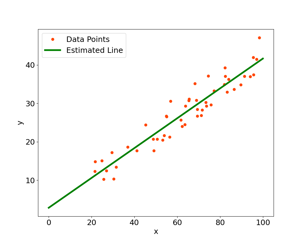
The estimated values that we obtain for $m$ and $b$ are $m \approx 0.38828$ and $b \approx 2.81487$. These values are close to the values we set (i.e. $m=0.4$ and $b=3$) and the difference comes from the fact that we added an error term (i.e. some noise) to the data. The final plot can be found below, click to enlarge.

The linear regression problem can also be defined for more than one indepedent variable and the equations are typically written in matrix form. For a generic point with output $y_i$ then there are $p$ different input variables and each of them is associated to a specific $\beta$ coefficient and $\beta_0$ is the intercept. The equation for a generic $i$ data point is: \begin{equation} y_i=\beta_0+\beta_{1}x_{i1}+\beta_{2}x_{i2}+\cdots+\beta_{p}x_{ip}+\epsilon_i \end{equation}

This can be written in matrix form, taking into account all $n$ data points, in this way: \begin{equation} \boldsymbol{y}=\boldsymbol{X\beta}+\boldsymbol{\epsilon} \end{equation} Where: \begin{equation} \boldsymbol{y}= \begin{bmatrix} y_1 \\ y_2 \\ \vdots \\ y_n \end{bmatrix} \boldsymbol{\beta}= \begin{bmatrix} \beta_0 \\ \beta_1 \\ \vdots \\ \beta_p \end{bmatrix} \boldsymbol{\epsilon}= \begin{bmatrix} \epsilon_1 \\ \epsilon_2 \\ \vdots \\ \epsilon_n \end{bmatrix} \end{equation} \begin{equation} \boldsymbol{X}= \begin{bmatrix} 1 & x_{11} & \cdots & x_{1p} \\ 1 & x_{21} & \cdots & x_{2p} \\ \vdots & \vdots & \ddots & \vdots \\ 1 & x_{n1} & \cdots & x_{np} \end{bmatrix} \end{equation} The coefficients can be estimated with the inputs and outputs by using the formula below: \begin{equation} \hat{\boldsymbol{\beta}}=\boldsymbol{(X^TX)^{-1}X^Ty} \end{equation}

The first step to code a multiple linear regression problem is again to import the numpy library for matrix calculations and the generation of random numbers, then $n$ datapoints need to be generated within a certain range, the coefficients $\boldsymbol{\beta}$ need to be set to some values that we will try to estimate and then some noise (i.e. error $\boldsymbol{\epsilon}$) needs to be added.

import numpy as np

# Multiple Linear Regression
n=100 #Number of datapoints
dim=10 #Number of inputs
min_value=20
max_value=100
error=5

np.random.seed(0) #Set seed to 0 to reproduce the results
x0=np.ones(n) # Input for intercept
#Generate random values within min_value and max_value for all inputs
x_inputs=min_value+np.random.rand(n,dim)*(max_value-min_value)
#Create matrix X
x=np.column_stack((x0,x_inputs))

#Randomly generate the true coefficients of inputs+intercept
#The coefficients are rounded for readability
beta=10*np.round(np.random.rand(dim+1),2)
#Print coefficients
print("beta: ",beta)

#Create the output vector and add the error
y=np.matmul(x,beta)+(np.random.rand(n)-0.5)*2*error

Now that the datapoints are generated we can use Equation 7 mentioned before to estimate the values of the coefficients $\boldsymbol{\beta}$ by using the generated data which also have an error term. We can also calculate the RMSE (Root Mean Squared Error) and R2 to understand how good is the fit.

#Estimate the coefficients by using the linear regression formula
beta_estimate=np.linalg.inv(x.T.dot(x)).dot(x.T).dot(y)
#Print coefficients
print("beta_estimate: ",beta_estimate)

#Calculate the estimated outputs with the estimated coefficients
y_estimated=np.matmul(x,beta_estimate)

#Calculate RMSE and R2 and print them
e=y-y_estimated
rmse=np.sqrt(sum(np.power(e,2))/n)
print("RMSE: ",rmse)
RSS=sum(np.power(e,2))
y_mean=np.mean(y)
TSS=sum(np.power(y-y_mean,2))
R2=1-RSS/TSS
print("R2: ",R2)

The output obtained in the console by running this script is the following:

beta:  [5.9 0.1 4.8 7.1 0.4 8.8 5.2 0.3 2.2 9.5 5.8]
beta_estimate:  [6.02112499 0.12400701 4.76326786 7.07496647 0.38437596 8.7953499
 5.22227853 0.30476328 2.19547803 9.53024073 5.79698863]
RMSE:  2.776292953816994
R2:  0.9999574652030081

The results show the true generated coefficients and the estimated coefficients, their value is quite close. They do not converge to the exact values because we added an error term which is added to the output but it is not represented by the known coefficients that are optimized, so the values of the known coefficients are estimated to optimally compensate for this error.

In the console, by printing the first 10 values for y and y_estimated we again notice that they are close to each other.

y[0:10]
Out[1]: 
array([3169.50344355, 2677.83957315, 2599.45249672, 2888.86318294,
       2642.51089869, 2369.6584953 , 2318.21475752, 2497.55733694,
       2519.94184974, 2173.6139939 ])

y_estimated[0:10]
Out[2]: 
array([3173.52503944, 2679.09973339, 2599.44422339, 2893.44085692,
       2642.94022617, 2368.85493225, 2322.09307819, 2494.95938554,
       2517.36137431, 2176.14174951])

The fact that the estimated coefficients are a good fit is also confirmed by RMSE and R2: RMSE is around $2.78$ which is quite small considering that the output is in the order of several thousands and R2 is really close to 1 which implies that most of the variance of the dependent variable is explained by the known independent variables.

Click the button below to see how to code linear regression using the scikit-learn library to predict house prices.

LR Prices Predictions

This is another example problem where is predicted if an electric car is able to complete a long journey. The page links to my Youtube video on my official channel.

LR Example Problem

	r/ValianTek_World
Code of Linear Regression created from scratch in Python using only main equations
|View Comments|Write Comments|