Linear Regression is used to find linear functions and a line, in a single-dimension form (i.e. single input $x$), has two coefficients which we can call $m$ and $b$: $m$ modifies the slope of the line while $b$ is called 'intercept' and it is the value of the output $y$ when all the explanatory variables (i.e. input values) are equal to 0. In case of a single input the linear function is $y=mx+b$. Figure 1 shows $m$ and $b$.

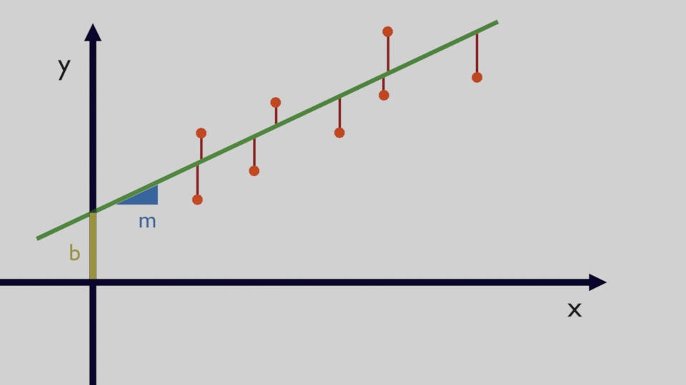
The main task in a Linear Regression problem is to find the coefficients which, as whown in Figure 1, are able to create a line where the difference between the known data (orange dots) and the line is as small as possible. These differences (shown in red) are called "residuals" and they need to be minimized. Let's imagine that there are $n$ datapoints and the $i^{th}$ datapoint $x_i$ is associated to the output $y_i$, the line formula is $y_i=mx_i+b+\epsilon_i$ where $\epsilon_i$ is an an error term which takes into account all the variations of the output which are not associated to the known input variables.

This problem can be solved by using a procedure called Ordinary Least Squares (OLS) where the sum of all the squared residuals mentioned before are minimized. Mathematically this means: \begin{equation} \min_{\hat{m},\hat{b}} \sum_{i=1}^{n} (y_i-\hat{m}x_i - \hat{b})^2 \end{equation}

The idea, as you can see in the equation above, is that the squared residuals are summed together for all $n$ data points and by finding the optimal $m$ and $b$ coefficients this final sum can be optimally minimized. Or, in other words this final sum of squared differences between the predicted and the observed values, can be minimized. Note that the $m$ and $b$ coefficients found are estimates so we call them respectively $\hat{m}$ and $\hat{b}$ however for the rest of this explanation they simply be called $m$ and $b$ to simplify the notation. To find $m$ and $b$, it is possible to use the following formulas: defining, $\bar{x}=\frac{\sum_{i=1}^{n}x_i}{n}$ and $\bar{y}=\frac{\sum_{i=1}^{n}y_i}{n}$, which are respectively the mean of $x$ and the mean of $y$ the formulas for $m$ and $b$ are: \begin{equation} m=\frac{ \sum_{i=1}^{n}y_i(x_i-\bar{x})}{\sum_{i=1}^{n}x_i(x_i-\bar{x})} \end{equation} \begin{equation} b=\bar{y}-m\bar{x} \end{equation}

So, after calculating $m$, the value can be used to calculate $b$. Click the button below to see the derivation of these formulas.

Linear Regression Math

The linear regression problem can also be defined for more than one indepedent variable and the equations are typically written in matrix form. For a generic point with output $y_i$ then there are $p$ different input variables and each of them is associated to a specific $\beta$ coefficient and then there is also the coefficient $\beta_0$ not associated to any variable because this is the intercept. The equation for a generic $i$ data point is: \begin{equation} y_i=\beta_0+\beta_{1}x_{i1}+\beta_{2}x_{i2}+\cdots+\beta_{p}x_{ip}+\epsilon_i \end{equation}

This can be written in matrix form, taking into account all $n$ data points, in this way: \begin{equation} \boldsymbol{y}=\boldsymbol{X\beta}+\boldsymbol{\epsilon} \end{equation} Where: \begin{equation} \boldsymbol{y}= \begin{bmatrix} y_1 \\ y_2 \\ \vdots \\ y_n \end{bmatrix} \boldsymbol{\beta}= \begin{bmatrix} \beta_0 \\ \beta_1 \\ \vdots \\ \beta_p \end{bmatrix} \boldsymbol{\epsilon}= \begin{bmatrix} \epsilon_1 \\ \epsilon_2 \\ \vdots \\ \epsilon_n \end{bmatrix} \end{equation} \begin{equation} \boldsymbol{X}= \begin{bmatrix} 1 & x_{11} & \cdots & x_{1p} \\ 1 & x_{21} & \cdots & x_{2p} \\ \vdots & \vdots & \ddots & \vdots \\ 1 & x_{n1} & \cdots & x_{np} \end{bmatrix} \end{equation}

Given that there are $n$ data points, $\boldsymbol{y}$ is a vector of $n$ by 1 dimensions and also the error term $\boldsymbol{\epsilon}$ is a vector of $n$ by 1 dimensions. On the other hand, $\boldsymbol{\beta}$ as previously mentioned is a vector of $p+1$ by 1 dimensions where $p$ is the number of input variables and then we add the intercept. For the data, this is a matrix of $n$ by $p+1$ dimensions given that there are $n$ data points but for each data point there is a multiplication for the $\boldsymbol{\beta}$ vector of coefficients which is $p+1$ dimensions. In the matrix one column is all ones, that is the intercept column which multiplies the $\beta_0$ coefficient and this is a compact way to include the intercept in the input matrix.

The Ordinary Least Squares (OLS) defined in matrix form is similar to the 1-dimension case. The equation below shows how the problem is formally posed and that is essentially the same equation used previously where the sum of all the squared residuals is calculated and then minimized but in this case the aim is to find a vector $\boldsymbol{\beta}$ with all its $p+1$ coefficients. \begin{equation} \min_{\boldsymbol{\beta}}\|\boldsymbol{y-X\beta}\|^2 \end{equation} Also this problem in matrix form can be solved with a closed form expression which is: \begin{equation} \hat{\boldsymbol{\beta}}=\boldsymbol{(X^TX)^{-1}X^Ty} \end{equation} The expression shows that by simply doing some transpose, inversions and matrix multiplications of the input data and the output it is possible to obtain the optimal estimate $\hat{\boldsymbol{\beta}}$ which are the coefficients of the linear regression problem. Click the button below to see the derivation of this formula.

Linear Regression Math