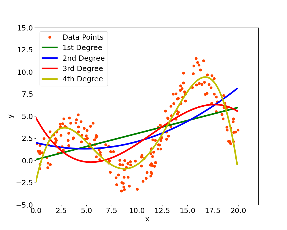
Polynomial Regression is used to find non-linear functions that are able to fit the provided data. In particular, the methodology finds the coefficients of an p-th degree polynomial which is able to represent the data. The user selects the degree $p$ of the poynomial: in case of $p=1$ this becomes a Linear Regression, with $p=2$ becomes a quadratic function, with $p=3$ becomes cubic and so on. Figure 1 shows how the selection of the degree affects the function: a low degree might be unable to describe the data while an high degree increases the complexity of the function and it can overfit the data, it is important to try different degrees and select the one that better represents the provided data.

In the general case, the output $y_i$ is described by the p-th degree polynomial shown in Equation 1. \begin{equation} y_i=\beta_0+\beta_{1}x_{i}+\beta_{2}x_{i}^2+\cdots+\beta_{p}x_{i}^p+\epsilon_i \end{equation} The equation is similar to the Linear Regression one but in this case every term of the polynomial is considered as an independent variable and each term is associated to a specific $\beta$ coefficient and then there is also the coefficient $\beta_0$ not associated to any variable because this is the intercept: while in the case of linear regression there is a single feature associated to a certain coefficient here you have the same feature repeated multiple times but with different exponents such as $x$, $x^2$, $x^3$, and so on. The Equation 1 shows an example where there is a single feature with different exponents, this can be generalized further by adding other features but overall the math is the same. The term $\epsilon_i$ is an an error term which takes into account all the variations of the output which are not associated to the known input variables. Click the button below to see how similar Polynomial Regression is to Linear Regression.

Intro to Linear Regression

Given that the equation is still linear in the coefficients, and the only difference is to consider non-linear inputs as independent variables, the problem to find the optimal values of the $\beta$ coefficients can be solved using the same procedure used in Linear Regression which is Ordinary Least Squares (OLS): the sum of all the squared residuals (i.e. differences between actual and predicted values) are minimized. The section below shows the equations in matrix form and the formula used to find the coefficients.

The polynomial regression problem is typically written in matrix form due to the number of independent variables (i.e. terms of the polynomials) used. The Equation 1 mentioned before can be written in matrix form, by taking into account all $n$ data points, in this way: \begin{equation} \boldsymbol{y}=\boldsymbol{X\beta}+\boldsymbol{\epsilon} \end{equation} Where: \begin{equation} \boldsymbol{y}= \begin{bmatrix} y_1 \\ y_2 \\ \vdots \\ y_n \end{bmatrix} \boldsymbol{\beta}= \begin{bmatrix} \beta_0 \\ \beta_1 \\ \vdots \\ \beta_p \end{bmatrix} \boldsymbol{\epsilon}= \begin{bmatrix} \epsilon_1 \\ \epsilon_2 \\ \vdots \\ \epsilon_n \end{bmatrix} \end{equation} \begin{equation} \boldsymbol{X}= \begin{bmatrix} 1 & x_{1} & \cdots & x_{1}^p \\ 1 & x_{2} & \cdots & x_{2p}^p \\ \vdots & \vdots & \ddots & \vdots \\ 1 & x_{n} & \cdots & x_{n}^p \end{bmatrix} \end{equation}

Given that there are $n$ data points, $\boldsymbol{y}$ is a vector of $n$ by 1 dimensions and also the error term $\boldsymbol{\epsilon}$ is a vector of $n$ by 1 dimensions. On the other hand, $\boldsymbol{\beta}$ as previously mentioned is a vector of $p+1$ by 1 dimensions where $p$ is the degree of the polynomial (i.e. it can also be seen more generally as the number of input variables) and then we add the intercept. For the data, this is a matrix of $n$ by $p+1$ dimensions given that there are $n$ data points but for each data point there is a multiplication for the $\boldsymbol{\beta}$ vector of coefficients which is $p+1$ dimensions. In the matrix one column is all ones, that is the intercept column which multiplies the $\beta_0$ coefficient and this is a compact way to include the intercept in the input matrix.

The equation below shows how the problem is formally posed in the Ordinary Least Squares (OLS) procedure and that is essentially shows that the sum of all the squared residuals is calculated and then minimized to find a vector $\boldsymbol{\beta}$ with all its $p+1$ coefficients. \begin{equation} \min_{\boldsymbol{\beta}}\|\boldsymbol{y-X\beta}\|^2 \end{equation} Also this problem in matrix form can be solved with a closed form expression (the same used in Linear Regression) which is: \begin{equation} \hat{\boldsymbol{\beta}}=\boldsymbol{(X^TX)^{-1}X^Ty} \end{equation} The expression shows that by simply doing some transpose, inversions and matrix multiplications of the input data and the output it is possible to obtain the optimal estimate $\hat{\boldsymbol{\beta}}$ which are the coefficients that multiply the polynomial terms and solve the Polynomial Regression Problem. Click the button below to see the derivation of this formula from the OLS minimization problem in Linear Regression.

Linear Regression Math