The polynomial regression is used to fit the coefficients of a polynomial function to the provided $n$ datapoints. More specifically, the output $y_i$ is described by the p-th degree polynomial shown in Equation 1 where the $\beta$ coefficients multiply the polynomial terms and an error $\epsilon$ (not described by the input values) is included. \begin{equation} y_i=\beta_0+\beta_{1}x_{i}+\beta_{2}x_{i}^2+\cdots+\beta_{p}x_{i}^p+\epsilon_i \end{equation} The main task is to find the $\beta$ coefficients and this problem is typically written in matrix form in the following way: \begin{equation} \boldsymbol{y}=\boldsymbol{X\beta}+\boldsymbol{\epsilon} \end{equation} Where: \begin{equation} \boldsymbol{y}= \begin{bmatrix} y_1 \\ y_2 \\ \vdots \\ y_n \end{bmatrix} \boldsymbol{\beta}= \begin{bmatrix} \beta_0 \\ \beta_1 \\ \vdots \\ \beta_p \end{bmatrix} \boldsymbol{\epsilon}= \begin{bmatrix} \epsilon_1 \\ \epsilon_2 \\ \vdots \\ \epsilon_n \end{bmatrix} \end{equation} \begin{equation} \boldsymbol{X}= \begin{bmatrix} 1 & x_{1} & \cdots & x_{1}^p \\ 1 & x_{2} & \cdots & x_{2p}^p \\ \vdots & \vdots & \ddots & \vdots \\ 1 & x_{n} & \cdots & x_{n}^p \end{bmatrix} \end{equation}

This problem can be solved with the same closed form expression used in Linear Regression because the equation is still linear in the coefficients and the different terms of the polynomial are simply seen as separate inputs. The formula is: \begin{equation} \hat{\boldsymbol{\beta}}=\boldsymbol{(X^TX)^{-1}X^Ty} \end{equation}

The first step to code the polynomial regression problem is to import the numpy library for matrix calculations and the generation of random numbers and the matplotlib library for the plot of the results, then $n$ datapoints need to be generated within a certain range, the coefficients $\boldsymbol{\beta}$ need to be set to some values that we will try to estimate and then some noise (i.e. error $\boldsymbol{\epsilon}$) needs to be added.

import numpy as np
import matplotlib.pyplot as plt

# Polynomial Regression
n=50 #Number of datapoints
deg=3 #Polynomial degree
min_value=-3
max_value=3
error=10

np.random.seed(100) #Set seed to 100 to reproduce the results
x0=np.ones(n) # Input for intercept
#Generate random values within min_value and max_value for the first input
x1=min_value+np.random.rand(n)*(max_value-min_value)
#The other inputs are just powers of the original input
x=np.tile(x1,(deg,1)).T
for i in range(1,deg):
    x[:,i]=x[:,i]**(i+1)   
#Create matrix X by adding intercept
x=np.column_stack((x0,x))

#Randomly generate the true coefficients of inputs+intercept
#The coefficients are rounded for readability
beta=10*np.round(np.random.rand(deg+1),2)-5
#Print coefficients
print("beta: ",beta)

#Create the output vector and add the error
y=x.dot(beta)+(np.random.rand(1,n)[0]-0.5)*2*error

Now the datapoints are generated and Equation 5 mentioned before is used to estimate the values of the coefficients $\boldsymbol{\beta}$ by using the generated data which also have an error term. We can also calculate the RMSE (Root Mean Squared Error) and R2 to quantitatively understand how good is the fit.

#Estimate the coefficients by using the linear regression formula
beta_estimate= np.linalg.inv(x.T.dot(x)).dot(x.T).dot(y)
#Print coefficients
print("beta_estimate: ",beta_estimate)

#Calculate the estimated outputs with the estimated coefficients
y_estimated=x.dot(beta_estimate)

#Calculate RMSE and R2 and print them
e=y-y_estimated
rmse=np.sqrt(sum(np.power(e,2))/n)
print("RMSE: ",rmse)
RSS=sum(np.power(e,2))
y_mean=np.mean(y)
TSS=sum(np.power(y-y_mean,2))
R2=1-RSS/TSS
print("R2: ",R2)

The output obtained in the console by running this script is the following:

beta:  [ 4.8  3.8 -1.4  1. ]
beta_estimate:  [ 4.1040973   3.33156732 -1.35928847  1.05782705]
RMSE:  5.120423348170949
R2:  0.9326226992544419

The results show the true generated coefficients and the estimated coefficients and most of the values are close to the original ones, this is confirmed by R2 close to 1 and a quite small RMSE if compared to the They cannot converge to the exact values due to the error term which is added to the output but it is not represented by the known coefficients that are optimized, so the values of the known coefficients are estimated to optimally compensate this error.

In the console, by printing the first 10 values for y and y_estimated we again notice that they are overall the estimated values are close to the original values in several cases.

y[:10]
Out[1]: 
array([  2.80825514,  -8.27651753,  -3.7394326 ,  10.27619038,
       -54.20119367, -22.64350887,   5.82400179,  16.20747303,
       -17.89296742,  -0.8286062 ])

y_estimated[:10]
Out[2]: 
array([  4.89822906,  -5.2172989 ,   2.21817412,  14.54350885,
       -45.56032657, -22.85146436,   7.22805499,  13.32740528,
       -20.57210586,   5.42598159])

This is also confirmed by RMSE and R2: RMSE is around $5.12$ which is relatively small if compared to the fact that the output roughly spans from -50 to 20 and R2 has a value close to 1 which implies that most of the variance of the dependent variable is explained by the known independent variables. R2 is typically used in Linear Regression but it can be used here because the equations are linear in the coefficients that are estimated.

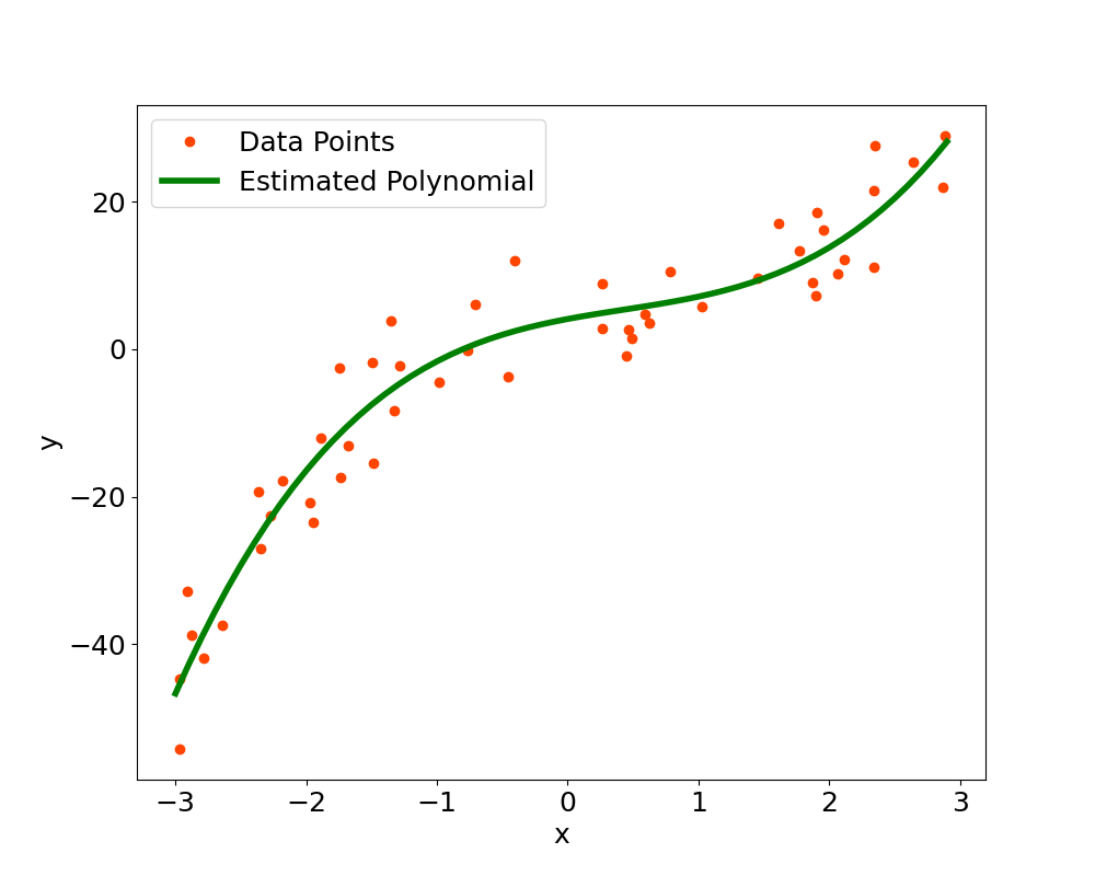
The final step is to plot the datapoints and then the estimated polynomial in $x$ (we remember that the original input data is only $x$, all the other inputs are powers of $x$).

#Plot the datapoints
plt.figure(figsize=(10, 8))
plt.plot(x[:,1], y, color='orangered',marker='o',linestyle='none',label='Data Points')
#Generate points with step stp between min_value and max_value
step=0.1
x1_plot=np.arange(min_value,max_value,step)
#Create intercept with the same length of the generated points
x0=np.ones(len(x1_plot))
#Create the other degrees
x=np.tile(x1_plot,(deg,1)).T
for i in range(1,deg):
    x[:,i]=x[:,i]**(i+1)   
#Create matrix X_plot by adding intercept
x_plot=np.column_stack((x0,x))
#Calculate the estimated plot outputs with the estimated coefficients
y_plot_estimated=x_plot.dot(beta_estimate)
#Plot the estimated polynomial
plt.plot(x1_plot,y_plot_estimated,'g',linewidth=4,label='Estimated Polynomial')
plt.tick_params(labelsize=18)
plt.xlabel("x",fontsize=18)
plt.ylabel("y",fontsize=18)
plt.show()
plt.legend(fontsize=18)

The plot also visually confirms that the estimated polynomial function is able to fit the data, as can be seen in Figure 1.