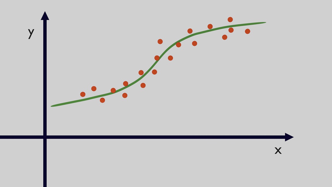
The main objective in regression problems is to find a function that is able to fit the data. This essentially means to have a function which outputs a prediction $y_{pred}$ given input data $x$ and the value of $y_{pred}$ should be as close as possible to the actual value $y$ ($y$ and $x$ are respectively called dependent and independent variable). Several machine learning methodologies can be used to find this function. The example shown is for a single dimension but the concept is the same in case of data with more than one dimension. Given some points, as shown in Figure 1, the solution of a regression problem is a function close to the data.

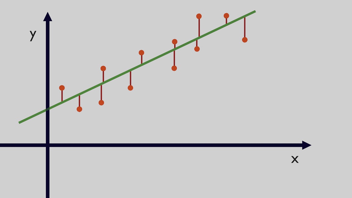
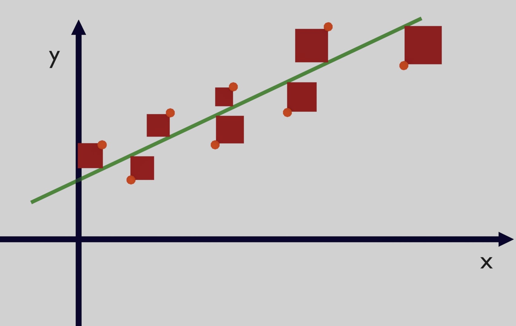
From a mathematical perspective, the goal is to reduce the difference between predictions, which is the output of the selected methodology, and the observed data points. These differences are called "residuals". The task is to reduce these residuals as much as possible. In Figure 2 you can see the main function in green and the residuals are the red lines between the observed points and the function.

The goal is to reduce the residuals which are calculated as difference between an actual value $y$ and the predicted value $y_{pred}$ of the function that fits the data, so $\epsilon=y-y_{pred}$. The table below shows an example of actual and predicted values and the associated residuals which can be positive or negative given that the function can underestimate or overestimate the actual values.

Actual Value	Predicted Value	Residual
4	3.8	0.2
6.5	7	-0.5
3.7	2.9	0.8
8.2	7.6	0.6
2	2.4	-0.4

Mean Absolute Error

The idea behind a metric is to have a number which summarizes the performance of the selected function. A possible metric is the Mean Absolute Error (MAE). This metric sums the absolute value of the residuals and this sum is divided by the number of residuals to get an average, the mathematical formula can be seen in Equation 1. It is worth noticing that the absolute value is used because we want to sum the magnitudes of all the residuals, if you leave negatives and positive residuals they cancel out giving the false impression that the error is small. The absolute residuals from the table above are $[0.2,0.5,0.8,0.6,0.4]$ and the MAE is the average of these values so $MAE=0.5$. \begin{equation} MAE=\frac{1}{n}\sum_{i=1}^n |\epsilon_i| \end{equation}

Root Mean Squared Error

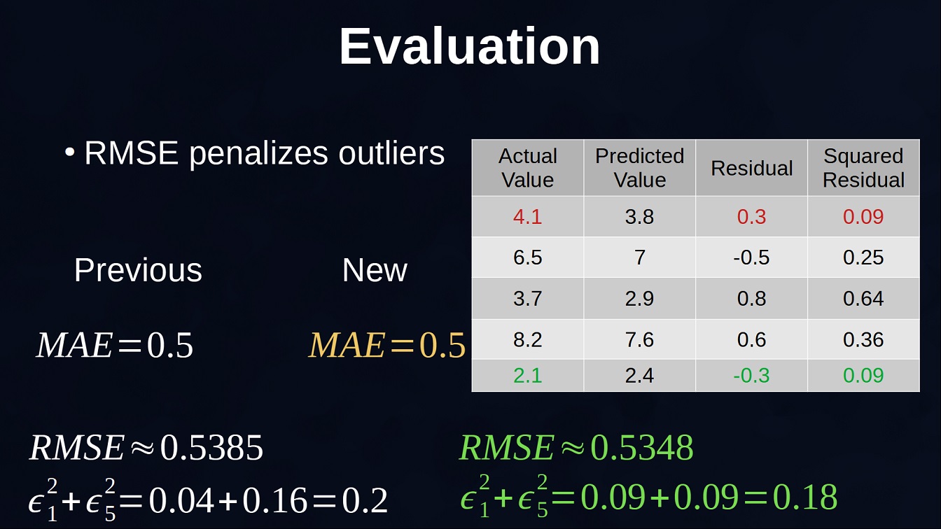
Another metric typically used is called Root Mean Squared Error (RMSE). Here instead of using the absolute value of the residuals, the values are squared so also in this case they are all going to be positive values. Then the square root is used on the mean of these squared residuals in order to have the same units of the variable of interest, formula in Equation 2. The main difference with MAE is that by squaring the values, the errors of the outliers increases. Essentially, this metric gives a high weight to large errors so the outliers, which are points with residuals typically much larger than the rest of the points, can influence more this metric value. The squared residuals from the table above are $[0.04,0.25,0.64,0.36,0.16]$ and then $RMSE \approx 0.538$. \begin{equation} RMSE=\sqrt{\frac{\sum_{i=1}^n (\epsilon_i)^2}{n}} \end{equation} This can be shown with the example in Figure 3. Here we increase the first point from 4 to 4.1 and increase the last point from 2 to 2.1. Given that the first point was understimated and the last point was overestimated we have essentially increased the distance from the prediction by 0.1 in the first case and reduced by the same amount in the second case. As a result, given that Mean Absolute Error threats all the values equally, the new value remains the same. 0.5. On the other hand, previously the squared residuals for the first and last point were respectively 0.04 and 0.16 for a total of 0.2. You can see that the increment of the first point is smaller than the decrement of the second point and the total sum is 0.18 which is smaller than 0.2 and for this reason the final value of the RMSE is smaller.

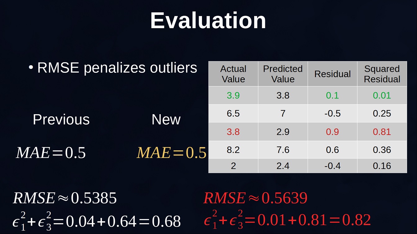
In this other example in Figure 4 we see the opposite scenario. The first point is decreased from 4 to 3.9 while the third point is increased from 3.7 to 3.8. The Mean Absolute Error still has the same value but, for the RMSE, by further increasing the distance of the outlier the sum of the first and third squared residuals goes from 0.68 to 0.82 and this results in an increased RMSE. In case outliers need to be reduced and taken into account more than the rest of the points RMSE is typically a better choice.

Mean Squared Error

The Mean Squared Error (MSE) is related to the Root Mean Square Error but it does not calculate the square root. In this case the units are squared so they cannot be directly compared to the variable of interest and there is not a direct interpretation of the result, however in case the metric is used just to compare the performance of two functions the user might be simply interested in which one has the smallest value and instead of using the Root Mean Square Error it is possible to use the Mean Square Error and avoid to calculate the square root. Equation 3 shows the formula of the MSE. \begin{equation} MSE=\frac{\sum_{i=1}^n (\epsilon_i)^2}{n} \end{equation}

All these metrics range from 0 to infinity where 0 is the best value which means that all the residuals have value 0. Software packages already include all these metrics and you can select the one more suitable for your problem. Next section describes the R-Squared metric.

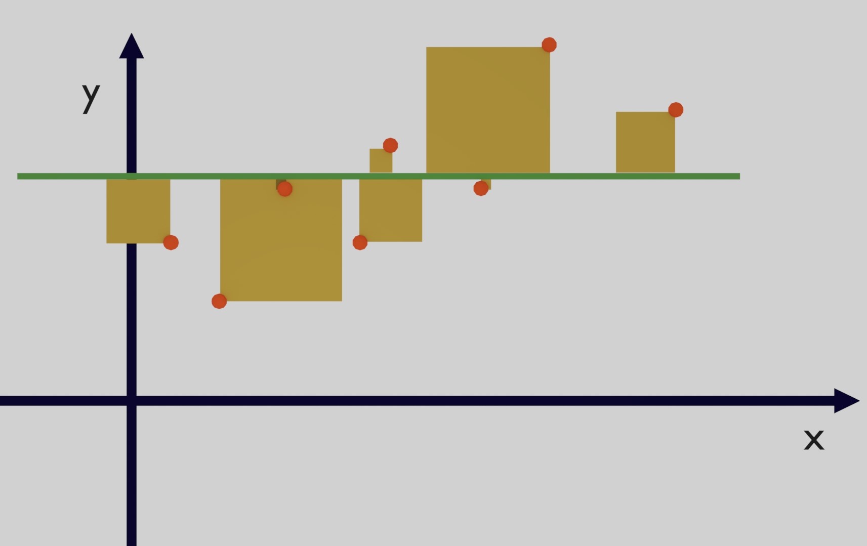
R-Squared is mainly used in Linear Regression problems where there is a linear relationship between the input and the output. This metric quantifies the amount of variance of the dependent variable which can be predicted by the independent variable. To calculate this metric we need to first calculate the total sum of squares (TSS): this is essentially the sum of the squared differences between the points and the mean of all the points. The formulas can be seen in Equations 4 and 5.

\begin{equation} \bar{y}=\frac{1}{n}\sum_{i=1}^n y_i \end{equation} \begin{equation} TSS=\sum_{i=1}^n (y_i-\bar{y})^2 \end{equation}

In Figure 5 the total sum of squares is the sum of all the yellow squares.

Then, the second step is to calculate the residual sum of squares (RSS) which is similar to the Mean Squared Error but without calculating the mean (Equation 6). Essentially these are the squared error of the functions that we believe is a good fit for the data. \begin{equation} RSS=\sum_{i=1}^n (\epsilon_i)^2 \end{equation} In Figure 6 the residual sum of squares is the sum of all the red squares.

The third and final step is to calculate R-Squared which is 1 minus the ratio between the residual sum of squares and the total sum of squares, as shown in Equation 7. \begin{equation} R^2=1-\frac{RSS}{TSS} \end{equation} This metric typically goes from 0 to 1:

• If the function is a perfect match for the points the residual sum of squares is 0 and the R-Squared is 1 which is the best value.
• If the selected function is not able to provide better results than the horizontal line which is simply the mean of the data, then the ratio is close to 1 and R-Squared is close to 0.

In particular cases the function selected is very bad and the sum of all residuals is greater than the mean of the data and this means that the ratio is also greater than 1 and R-Squared becomes negative and this type of function should be discarted because it is not a good representation of the data. Comparing the squares of the two figures we can see that the function selected is a good fit because the red squares are quite small in comparison to the yellow squares obtained with the mean of the data. This is simply a visual comparison but the point of using R-Squared is that we can quantify how well a function fits the data.

	r/ValianTek_World
Details and formulas of some common Regression Metrics: MAE, RMSE, MSE, R2
|View Comments|Write Comments|